


 Bishop Hill
 Ed's evidence of low TCR
Climate: sensitivity This is a guest post by Nic Lewis.
As many readers will know, there is a lengthy and pretty civilised discussion of the recent Lewis/Crok report ‘A Sensitive Matter’ on Ed Hawkins' blog Climate Lab Book, here. In that report, we gave a 'likely' (17-83% probability) range for the transient climate response (TCR) of 1.0°C to 2.0°C. TCR is more relevant to warming over the rest of this century than equilibrium climate sensitivity (ECS).
The guest post by Piers Forster that headed the Climate Lab Book thread made the mistaken claim:
Particularly relevant, is our analysis in Forster et al. (2013) that confirms that the Gregory and Forster (2008) method employed in the Lewis & Crok report to make projections (by scaling TCR) leads to systematic underestimates of future temperature change (see Figure 1), especially for low emissions scenarios, as was already noted by Gregory and Forster (2008).
However, that wasn't really Piers' fault as he had, I believe, probably gained an incorrect understanding as to the method used in our report from another climate scientist. After I pointed this out, Piers very properly backtracked later in the thread, writing:
Nic’s pipeline factor may correct the underestimate, or it may not. I don’t think we have any way of knowing. To me this gets to the nub of my point on assumptions. I’m not really trying to say Nic’s results are wrong. I’m just trying to show that model and assumption choices have a huge effect as there is no perfect “correct” analysis method.
I agree that there is no perfect ‘correct’ analysis method for TCR and ECS. But there are plenty of studies using methods and/or data that are clearly incorrect, and whose results should therefore be discounted, as the authors of the IPCC AR5 report did for some methods and we did in the report in relation to certain studies. Some people have accused us of cherry picking – or as AR5 WGI co-chair Thomas Stocker put it in the newspaper Die Weltwoche, according to Google Translate:
He criticized the authors have picked them agreeable studies as raisins.
However, in fact I had identified serious shortcomings in all the ECS and TCR studies used in AR5 that we discounted, as described here.
Returning to Ed Hawkins, in his comments at Climate Lab Book he wrote:
As Piers’ post points out, there is evidence that the approach adopted by Lewis & Crok is sensitive to decisions in the methodology and may underestimate TCR.
which perhaps puts a slant on Piers' position.
That brings me to the main point of this post. Ed Hawkins has recently had a new study accepted by Journal of Climate (pay-walled). Congratulations, Ed. Being a scientist not a politician, I don't believe in making knee-jerk reactions to lengthy, detailed work. So I won't criticise Ed's study until I have thoroughly read and digested it, and then only if I think it has serious shortcomings. However, I do have a few initial observations to make on it.
Ed's new study uses a small ensemble of versions of the Met Office HadCM3 climate model with different parameter settings, and hence varying ECS and TCR values. Although the study is mostly about evaluating and correcting decadal climate hindcasts, it also deduces a probabilistic estimate for TCR. It isn't yet clear to me whether the method is sound and the study's conclusions about TCR justified. But even assuming they are, given all the uncertainties involved and the use of a single climate model it seems appropriate to take the more conservative, wider, of the 5-95% ranges for TCR that the study gives (doubling the identified assumed errors).
So how does the more conservative 5–95% range for TCR given in Ed's study compare with the 17–83% range given in the Lewis/Crok report, which ‘may underestimate TCR’ according to him? Well, what do you know, his range is 0.9°C to 1.9°C – slightly lower than our 1.0°C to 2.0°C range. And much tighter, as his is a 5–95% range and ours only a 17–83% range.
So here's another study supporting our contention that the top of the IPCC's 17–83% range for TCR is much too high at 2.5°C. Indeed, almost half the CMIP5 models' TCR values given in AR5 exceed the conservative range 95% bound of 1.9°C in Ed Hawkins' new study – the newer Met Office HadGEM2-ES model being way above at 2.5°C.
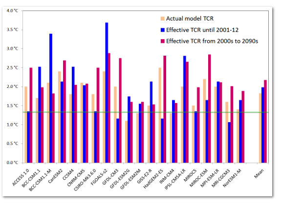
Moreover, most of the CMIP5 models used for the AR5 projections of climate change show significantly higher warming over the rest of the century than one might expect from their TCR values: their 'effective TCR' from the 2000s to the 2090s exceeds their actual TCR. Figure 8 of our study, reproduced below, shows this – compare the magenta and salmon bars.
 Effective TCRs for CMIP5 models analysed in Forster 2013
The salmon bars show model TCRs, estimated as per the definition of TCR, by increasing the CO2 concentration in the model by 1% p.a. for 70 years. The blue bars show TCR estimatesbased on model simulations over the instrumental period, to 2001–12, i.e. ‘effective historical’ model TCRs. The magenta bars show TCR estimates based on the subsequent change in model-simulated temperatures to 2091–99 on the RCP8.5 scenario, i.e. ‘effective future’ model TCRs. The multimodel means are shown at the right. The horizontal green line shows the observationally-based TCR best estimate of 1.35°C.

Reader Comments (50)
Will Ed get the point that rushed commentary isn't appropriate for a scientist?
omnologos
"Will Ed get the point..."
O, I rather think he will!
I will comment in more detail later, but for those who want to read all the (rather technical) details, I have put my copy of the preprint online without a paywall:
http://www.met.reading.ac.uk/~ed/home/hawkins_etal_2014_decbias.pdf
cheers,
Ed.
PS. Hopefully the comments on this post can be a pretty civil and useful technical discussion too?
Ed, many thanks for the link.
[Snip O/T]
I second Ed's request that the comments on this post be a civil and useful technical discussion, and thank him for putting a copy of his paper's preprint online.
Firstly, great to see interest in a rather technical and obscure paper! You can read all the details here.
Anyway, as Nic describes we use many simulations of different decades during the past 50 years with different versions of the HadCM3 GCM, which all have different values of TCR, to effectively infer which version best matches trends in global temperature. There are lots of technical details about how this comparison is done - a lot of care is needed to ensure this is done fairly.
Some initial comments:
(1) The best estimate for TCR in our study is 1.64K when using the HadCRUT4 observations (see Figure 13). Table 1 illustrates that for other observational datasets (ERA40, NCEP, GISTEMP) the best estimate for TCR is around 0.15K larger (between 1.75-1.82K).
(2) Our conservative (statistical) uncertainty when using HadCRUT4 observations is 0.9-1.9K. But, this does not include possible systematic uncertainties which we cannot yet estimate, and could be of either sign. These are discussed in Section 5. The uncertainty bounds are also shifted upwards for the other observational datasets.
(3) Also note that the relationship between our measure of bias and TCR (Figure 13) could also be due to the different aerosol forcings in the different versions of the models (also shown in Figure 13). Nic has also done a lot of work on this aspect already but didn't discuss this in the post. This is a large caveat on our TCR constraint as we state in Section 5.
In summary:
Our median best estimate for TCR is between 1.64 and 1.82K (close to the IPCC average), depending on the observational dataset used. But, the uncertainty distributions are skewed with a slightly sharper cutoff for high TCRs. Our paper demonstrates that using HadCRUT4 can potentially result in an underestimate of TCR, when compared to other observation-based datasets. However, there are large caveats - mainly due to uncertainties in the forcings used, especially the aerosols.
So, it is essential when trying to estimate TCR to use a range of approaches because they all have different assumptions, caveats and possible systematic errors.
cheers,
Ed.
[Snip - O/T]
[Snip - O/T]
Heh, it's hard remaining civil while being dehumanized.
==============
And that's profoundly true kim.
Thanks for commenting, Ed.
I'll email you separately with some technical questions when I have had a more thorough look into your methods. I have it on my list to look at the aerosol forcing issue, which is particularly problematic for HadCM3. I concur with your statement in that connection, that "This is a large caveat on our TCR constraint". Whilst I didn't attempt to cover aerosol problems, in the post, I did refer to "all the uncertainties involved and the use of a single climate model".
The paper says that 'Unless otherwise stated we use HadCRUT4 in all that follows' and, as you say, I gave only the primary, HadCRUT4 based, conservative estimated TCR range. May I ask what the conservative 5-95% TCR ranges allowing doubled uncertainty in the true bias tendency are for the other surface temperature datasets – I don't think you give them in the paper?
You describe ERA40 and NCEP as observational datasets, but surely that isn't really correct – aren't they both just model-based temperature reanalyses that employ, but are not necessarily faithful to, observational datasets? Also, I'm not sure how good quality an observational dataset GISSTEMP is, with its dependence on extensive infilling and on at least one questionable reconstruction (for Byrd in Antarctica).
[Snip - O/T]
In Edinburgh there is a new library, The Library of Mistakes. I kid you not. It is related to the fields of finance and business, with the airm to increase understanding, by understanding past errors. A quote on the website is by James Grant, to the effect that progress is cyclical, not cumulative.
http://libraryofmistakes.com/
The concept is applicable to climate science.
[Snip - O/T]
No more discussion of the general topic of climate sensitivity please. Ed's paper only.
Hi Ed,
I have only just downloaded your paper and simply skimmed a little of the first part, so I am not in a position to make any proper comment. Nor do I have any expertise in the issue of TCR etc. However I do have expertise in other areas and one of these is the difficulty of determining non-stationary behaviour in real datasets. At superficial inspection, your paper is covering issues of bias (presumably in temperature reproduction) which are usually just subtracted out. You mention stationarity. You state:
Any assumption like that is to me an arbitrary decomposition into a non-stationary term, a bias term and a residual. The residual is then the part compared, for example, to temeprature series or other observations. The problem I can see is two-fold, firstly that the arbitrary decomposition allows a claim of high quality fit to external data, which is unjustified (I realise exploring this is one of the topics of the topic, so I am simply observing here, not criticising).
Secondly, and more importantly I think, what if there is long period variability in either the data or the model that is quasi-stationary but has a wavelength greater then at least half the observation window, but is the result of a physical effect in the real climate that you do not capture in a climate model? In such case you can arbitrarily make a non-stationary assumption and actually, detrend and obtain a fit even though the climate model fails to inlcude such a process.
How do you deal with this problem? If you use a linear de-trend, is the slope always positive or always negative or can it be either? What explicit assumptions do you make about stationary or non-stationary behaviour in the observations?
It was surprising to see that the 5-95% range was 1.4-1.8 for the true bias uncertainty, but that doubling the uncertainty moved the lower part of the range 5 times as far (to 0.9) as the upper part (only to 1.9 from 1.8). And then Figure 13 seems to explain this by a "fat tail" but to the LEFT (i.e. not in the direction of catastrophe). What a refreshing result!
The table shows what seems to me to be a pretty large reduction of the upper end, from 2.64 to under 2 for all four observational datasets. Yet Ed's comment above is "the uncertainty distributions are skewed with a slightly sharper cutoff for high TCRs". Slightly? Isn't it the difference between imminent disaster and a nice relaxed century or two to solve the problem?
knr -
Thank you, I was about to make a similar point, but I think Nic and Ed are to be congratulated for engaging in a grown-up debate with us lukewarmers (mostly) and seeking to give us an inside view on this topic. It is nice to see science in action as say Richard Feynman would recognise it. It doesn't matter whether either of you are right or wrong, it is the open, honest discourse that moves understanding forward, and the idea of a "settled" science that opposes it.
Thank you both.
Hi Nic,
Would be interested to hear your feedback on the paper. The conservative 5-95% ranges for the other three observation-based datasets are 1.2-2.0 or 1.2-2.1K, but skewed with medians close to 1.8K. These particular ranges were not quoted in the paper.
ERA-40 and NCEP reanalyses use the available observations and weather forecast models to constrain the state of the atmosphere. Your observational estimate of TCR also requires a model, but you do not always mention that. And, you agree that a range of methods are required for estimating TCR, and this is similarly true for different choices in how to reconstruct past temperatures - there is no perfect method so a diversity is used to explore the sensitivity to those choices.
cheers,
Ed.
Lance
"doubling the uncertainty moved the lower part of the range 5 times as far (to 0.9) as the upper part (only to 1.9 from 1.8). And then Figure 13 seems to explain this by a "fat tail" but to the LEFT"
I have to say that a fat tail on the left seems quite wrong to me given the physical and mathematical relationships involved. I would expect there to be a fat tail on the right if the major uncertainties have been properly allowed for. I haven't worked out yet why that isn't the case in Ed Hawkins' study.
The Sexton et al (2012) and Harris et al (2013) ECS and TCR studies underlying the UK climate projections [UKCP09], were like Ed Hawkins' study, based on a HadCM3 PPE [perturbed physics or perturbed parameter ensemble]. They used a far larger PPE, and likewise produced illogically shaped uncertainty distributions for TCR and ECS, but in their case with an almost Gaussian [normal] shape. However, those studies used methods that were completely unsuitable given the characteristics of HadCM3, and additionally applied a complex subjective Bayesian statistical analysis that will have biased the results in unknown ways. So their results are definitely worthless, at least if considered as observationally-based estimates.
Hi Nic,
I think the shape of the distribution comes from the fact that several models have a higher raw TCR than the best estimate, which allows a tighter constraint in that direction. Fewer models have a lower TCR than the best estimate.
Ed.
OK Ed, why can't you chuck out results from the worst models?
Ed, thanks for the link to your, as you quite rightly say " (rather technical) ." paper most of which I will struggle with, but to help me along the way could you please explain why :-
I was under the impression that "initialised" meant run from a point of known observational data?
Forgive me if I have missed it in the detail, if it is in there, could please just point to the section.
rhoda - I'm afraid you have missed the key point! By looking at the whole range of models and effectively weighting them by how well they perform you can actually constrain TCR better than if you just completely ignore some of them. Some of the models warm faster than observations and some warm slower than observations, so the true TCR must be in the middle somewhere.
Ed.
Green Sand - yes, we have deliberately chosen not to use the simulations initialised from observations. The term "initialised" can be used in a variety of ways - simulations can be "initialised" from observations or from model states. We are proposing quite a large change in how to best estimate the bias in retrospective predictions and so we wanted a simpler case to study first. Initialising with observations adds a whole new layer of complexity to estimating biases, but this is something that we hope to move on to looking at.
Ed.
What's the ratio of the ones that warm faster than observation to the one which run slower? It seems to me that if the ensemble as a whole runs warm, there is a case to chuck out the warmest. In modelling world are all models of equal value? That seems non-intuitive to me.
Thanks Ed
"Initialising with observations adds a whole new layer of complexity to estimating biases, but this is something that we hope to move on to looking at."
I think I get the complexities, volcanoes are obvious, others are more subtle and not so "clear cut". Basically at present you are looking at the "mechanics/methodology", only when initialising with observations will we get a clearer view of "actual" biases. Going to be interesting to watch.
Once again thanks, will go and read some more.
Hi Ed,
Thanks for your explanation about the shape of the distribution, which I see makes sense given your estimation method. I'll re-read your paper and think more about this before commenting further on this aspect.
You say "ERA-40 and NCEP reanalyses use the available observations and weather forecast models to constrain the state of the atmosphere. Your observational estimate of TCR also requires a model, but you do not always mention that. And, you agree that a range of methods are required for estimating TCR, and this is similarly true for different choices in how to reconstruct past temperatures."
Models are certainly needed - we do mention that in at least three places in the Lewis/Crok report, including in the Executive summary. However, I have a preference for where practicable using simple "models" – such as a few equations, or a straightforward way of deriving past temperatures from instrumental readings by some technique based on homogenising and combining separate records.
HadCRUT4 and (to somewhat lesser extent, due to infilling) NCDC MLOST and GISSTEMP involve fairly simple "models". You will find those surface temperature datasets included in Chapter 2 of AR5 under Changes in Temperature - Land and sea surface, but reanalyses such as ERA-40 and NCEP that use very complex models are not. I think there are good reasons for that.
Nic
Nic
You say that
I'd be most interested to know how you'd respond to this comment (set out below) by Pekka Pirila that I stumbled across the other day on And Then There's Physics when reading around the debate over your GWPF report.
Nic Lewis posts at 5.22 pm, Ed replies at 5.47 pm...
Rhoda posts a question at 5.46 pm, gets an answer from Ed at 5.50 pm...
Greensand posts at 5.50 pm, gets an answer from Ed at 5.57pm...
ThinkingScientist posts a question at 4.57 pm, gets no answer...
Hmmm...interesting. Is there an elephant in the room?
Good question, thinksci, there is no elephant, but there is a yet-to-be-determined number of angels dancing gracefully on pinheads.
Rhoda,
Richard Betts ignores my questions too. Perhaps they are stupid questions. Maybe they are inconvenient questions. They could be uncomfortable questions. I thought I asked nicely...
Ed,
I've now studied your paper further and have some initial thoughts on technical issues. It is possible that I have misunderstood some things, so please take these comments as tentative.
In HadCM3's standard configuration, total net anthropogenic radiative forcing increases by 1.15 W/m² between 1860 and 2000 and non-aerosol anthropogenic forcing (greenhouse gases, etc) by 2.25 W/m² (Gregory and Forster, 2008, Figure 2). Over 1960–2000, HadCM3's standard total net and total non-aerosol anthropogenic forcing increased by respectively 0.9 W/m² and 1.35 W/m². The corresponding best estimates from AR5 are 1.82 W/m² and 2.55 W/m² for 1860-2000, and 1.17 W/m² and 1.55 W/m² for 1960-2000. So it seems that HadCM3's anthropogenic forcing changes falls significantly short of the more recent and authoritative AR5 best estimates: they amount, as a percentage of the AR5 estimates, to 63% (88% ex aerosols) over 1860-2000, and to 77% (87% ex aerosols) over 1960-2000.
Your study uses the period 1961-2010 and 1961-2001, and does not separate out aerosol forcing. It seems, therefore, that the forcings used should be increased in proportion to 100%/77%, or thereabouts. You have assumed that the forcing trends in all PPE versions are the same. On that basis, wouldn't – at a first approximation – the effect of making this adjustment simply involve multiplying your TCR estimates by 0.77, since the forcing change appears in the denominator of the TCR calculation?
Making that adjustment would change your primary, HadCRUT4-based, median TCR estimate of 1.64 K (=°C) to 1.26 K, and that of 1.77 K using GISSTEMP to 1.36 K. Those figures are much more in line with other, properly observationally-based, TCR estimates that use forcing estimates consistent with those in AR5. Using the full AR5 probability distribution for anthropogenic forcing would probably restore a positive skew to your TCR estimate probability density [PDF].
However, I fear things are more complex. The assumption you make that forcing trends in all PPE versions are the same seems seriously wrong. See Figure B.1 in Box 1 of my analysis of the relationship between aerosol forcing and climate sensitivity in the HadCM3 PPE used in Harris et al (2013), available at http://niclewis.files.wordpress.com/2013/09/metoffice_response2g.pdf . The HadCM3 model exhibits a very strong increase in negative aerosol forcing for parameter combinations that result in a low ECS, and vice versa.
So I think that the 'True bias tendency' needs to be adjusted separately for each member of your PPE, by reference to how much its own forcing changes fall short of those in AR5, treating the AR5 forcing estimates probabilistically. That will change the regression relationships, although it is not clear to me that making these changes would give rise to the usual shape of an estimated TCR distribution.
I'll be interested in your reaction to my points. Whether or not your study can provide realistic estimates of TCR, its exploration of bias in decadal climate predictions seems to me worthwhile.
thinkingscientist
Er, excuse me - you seem to have forgotten me answering you only the other day, see here on Mar 13, 2014 at 12:13 AM, and again later at 7:59 PM.
:-)
Hi Richard,
I thought my comment would get you out of the woodwork. I could have said "Richard Betts always ignores my questions too" but I didn't, because you did answer a question last week. I said you ignore my questions, not all of them. You may have forgotten that I asked you the following questions. Three times. I am still waiting for the answers....They were addressed directly to you (twice) on the "Hopeful Fudging" thread see:
http://bishophill.squarespace.com/blog/2012/3/21/hopeful-fudging.html#comment17432322
they were posted in unthreaded and they were again posted to you on the "Quantifying Uncertainties in Climate Science" thread. On the latter thread you acknowledged the questions with:
Is a year long enough? O. Bothe did take the time to give excellent and very helpful responses with some good recommendations for reading. But I am still waiting for your answers. They are interestingly still reasonably pertinent questions on this thread:
You can answer them one at time if you like. :-). Q3 can now be ignored - O. Bothe kindly pointed out that that cannot be done (diffusion processes). Still looking forward to your answers. Or is it going to be as Dolphinhead said immediately after my point that you ignored the questions:
Just think of it as community outreach...
thinkingscientist - take a look at this paper, if you have not already seen it.
The Myopia of Imperfect Climate Models: The Case of UKCP09
Presumably heating the deep oceans involve a significant time lag. After all, it took years to come up with the idea that the missing heat is hiding there. Why would anyone bother to require a model of atmospheric temps to also show deep ocean temps?
As to the entire ensemble of models concepts: How is this significantly different from running a bunch of monkeys on typewriters and claiming that the occasional bits that might be interpreted as Shakespeare offers proof the monkeys are writing Shakespeare? It seems that selecting the good bits from many models only emphasizes that none of them are actually useful.
Nic Lewis - what is the origin of your radiative forcing numbers for the period 1860-2000 from both HadCM3 and IPCC AR5? I did not encounter these in AR5 WGI Chapter 8.
MArtin A - thanks I have downloaded it and will take a look. At least it clearly explains the acronyms and terminology!
How is this significantly different from running a bunch of monkeys on typewriters
The output of the monkeys is statistically independent. The models share assumptions and all sorts of other things.
hunter says: "Why would anyone bother to require a model of atmospheric temps to also show deep ocean temps?
"
Because the ocean and atmosphere are coupled in the models, as they are in the real world. The ocean is a huge heat sink (high heat capacity of water and huge mass) whereas the atmosphere has low heat capacity and mass. If your model does not couple them then the atmosphere would have much larger responses to forcing.
Splitpin & Hunter
The monkeys share the same PDF (the typewriter keyboard) and the same stationarity assumption. The CMIP5 models also share the same underlying parameters eg Milankovich forcing, scenarios for forcing etc. The different models are simply differently coded implementations of the same physics, with different emphasis/detail on various parts eg complexity or simplicity in some parameters.
The questions I have are related to the fundamental stationarity question. As I understand it the models are quasi-stationary unless external forcing is introduced. This appears apparent from the way the model "spin-up" from the CMIP5 time zero is presented, meaning all the models exhibit quasi-stationary behaviour unless the parameters containing the approved forcings are applied. This means all the models are essentially exhibiting stationarity in the physics and all the runs are simply stationary model physics + forcing trends. The problem with this is that it then makes very strong assumptions about the results of predictions from climate models:
(a) All the physics is accounted for and correct
(b) All the forcing mechanisms are accounted for (eg solar, volcanic, aerosols)
(c) All the forcing parameters are correctly quantified with time
The stationarity question is the key one to me. In Ed's paper he uses a Toy model to investigate the statistical bias aspect. The Toy model idea is fine, but the assumptions reinforce/emulate the model behaviour. The assumption is:
model result = quasi-stationary model from physics + linear forcing + stationary accumulating error terms
This derives from the assumption that, for example, the modern temperature record must comprise stationary physics + linear but time varying forcing profiles. Such a decomposition is arbitrary. The modern temperature record could be simply a chaotic physical process describing a random walk between stable boundary conditions and we simply don't understand all of the physical processes. The models really work like this:
Model result = quasi-stationary physics + sum of(multiple linear forcings with assumed time variant properties)
So if the models are run without forcing (except perhaps Milkankovitch) how do you keep them (a) stable and (b) are there are any emergent properties that show periodicities, and particularly intermediate and long period periodicities, eg 60 years, 1500 years? I think the last question is very important. Without answering that you cannot make any claims about the reliability of the models or their predictions.
Some examples of model problems:
1. The current hiatus in temperature. Not predicted by any climate model, multiple (sometimes conflicting) explanations as to its cause. Its been pointed out that models never show a hiatus of 20 years (and the probability of one the length we have currently observed is below 5%). At 20 years what will be the next excuse for the model prediction failure over this period?
2. Inability to predict the warming up to the 1940's, either in timing or magnitude.
Ben Lamkamp
"Nic Lewis - what is the origin of your radiative forcing numbers for the period 1860-2000 from both HadCM3 and IPCC AR5?"
As I wrote, for HadCM3 it is Gregory and Forster, 2008*, Figure 2. For AR5, look in Annex II, as stated in Chapter 8.
* Transient climate response estimated from radiative forcing and observed temperature change, JGR, 113, D23105
RichieRich
" I'd be most interested to know how you'd respond to this comment (set out below) by Pekka Pirila"
I'm afraid Pekka is wrong. He claims " Dropping the upper-air temperatures from the data set is an important difference between the two series of results and may have a big role in the change, possible the largest role." Yet, as I say in my paper, adding the upper air diagnostic hardly changes parameter inference. And although Pekka is stronger on Bayesian statistical issues, his objections to my objective prior aren't valid. It is an appropriate prior because it properly reflects data error distributions and other uncertainties. That can be seen by comparing results using the non-Bayesian profile likelihood method of inference, as used by some climate scientists, which involves no prior. They are almost the same as those using my objective Bayesian method, save for the ranges being a bit narrower (a known issue with profile likelihood).
The model used in my paper was necessarily the MIT 2D model, since that was what the Forest study I was reworking used. It may be a black box, like 3D GCMs are, but unlike them it does have calibrated control knobs for key climate system properties.
Hi Nic,
Firstly, the TCR estimates used come from the 1%/year increase in CO2 simulations, so should not be scaled, unless the GHG forcing trends vary a lot across the PPE ensemble.
I find it strange that you state that we assume all the forcings are the same across model versions. This is clearly incorrect.
Figure 13b shows exactly the data that you suggest we use! The relationship between TCR and true bias tendency could be due to the difference in aerosol forcings with the data coming from Harris et al. (2013). We also state that we cannot yet distinguish between the possibilities that the relationship is due to TCR or forcings, or both, and this will vary across model versions and shift the bias estimates. We do not state our TCR results in the abstract because we are not yet confident that this approach is providing a robust constraint. If this analysis was repeated across a wider range of models then we might be able to draw out some more robust constraints, or maybe not.
We have been very aware of the caveats, assumptions and limitations of our methodology - and this should be the same for any methodology.
cheers,
Ed.
thinkingscientist,
Thank you for the response regarding deep ocean coupling. I hope you don't mind if we explore this a bit further?
Here is whaat I am trying to get at:
Heat travels through the atmosphere in a multi-week or seasonal fashion- weather systems move in a matter of days and weeks. Het moving intot he deps should take quite a bit longer to not only get into the deeps, but to also get ack to where they can impact weather in any measurable way. Heat at 20000 meters below sea level is not going to do much if anything on weather. So to say the deep ocean heat is coupled to the atmosphere is to, as far as I can see, imagine a very spongy, llong delayed reaction sort of coupling. If the current understanding of El/La Nino/Nina is accurate, the winds pile up war water in the western Pacific, driving them down deep. When the winds weaken or reverse, the ehat is more well distributed, and is not driven so deeply. When the winds strengthen they can even bring relatively warm water towards the eastern Pacific, allowing more water vapor to move eastward into the Americas, etc. Does this proposed mechanism evn require deep ocean heat to happen, or is the easterly distribution of warmer surface waters sufficient? What is the proposed mechanism for bringing up this deep ocean resevoir? Hopefully it is more robust than the conjectures about the mechanism for the downward movement? But either way, is deep ocean heat moving down today even relevant for weather today?
splitpin,
Good point, but don't the keyboards offer a significant homogenizing restraint?
The point I was trying to make, however poorly, is that none of the models actually gets it right. Instead it seems the AGW apologists are taking bits and pieces. When one gets a good output from a model that happens to be good for a particular point in time the apologists are claiing that validates the entire ensemble. If this is correct, then it is not really so different from the monkeys flailing away on the keyboards, is it?
.
Hi Ed,
First, you find it strange that I state that you assume all the forcings are the same across model versions (actually I said that of the forcing trends in all PPE versions). I did so because you say in the paper, line 429:
"we have assumed that the forcing trends in each PPE version are the same".
Am I missing something here?
I think you misunderstood my point about scaling TCR values; maybe I didn't express it clearly enough. I know how the TCR values were derived. Since they depend on doubling the concentration of CO₂, what forcing that corresponds to is irrelevant. In the below explanation, I assume that the model-projected warming is proportional to the product of the model-version TCR value and the forcing applied in the model over the period concerned. The proportionality won't be exact, but I think this relationship will be approximately true. The constant of proportionality will depend on the period involved and on the model forcing corresponding to a doubling of CO₂. The near identity of the 1860–2000 increase in greenhouse gas forcing shown for HadCM3 in Gregory and Forster 2008 [GF08] and in AR5 indicate the latter is close to the value of 3.7 W/m² used for the AR5 forcing estimates.
However, suppose the standard model version with a TCR of 2.0°C exhibited a zero 'true bias tendency', but that it had 'start-time independent' errors in the forcing applied to the model, whether arising from anthropogenic aerosol forcing in the model differing from that in the real world or otherwise, such that the net forcing applied in the model was only 77% of the true forcing. Then the warming projected by the model would equal the warming which a model version with a TCR of 77% x 2.0°C = 1.54°C would have produced had the model applied the correct, real world, forcings. So the zero 'true bias tendency' would in that case imply an observationally-constrained best estimate for TCR of 1.54°C, not of 2.0°C (leaving aside evidence from any other model versions). I assume you would agree with that?
I then went on to make the point the difference between model and real-world forcing changes would vary with the model version. That is mainly because aerosol forcing is closely related to climate sensitivity in differently parameterised versions of HadCM3. So all the uncertainty bars in your Figure 13.a) would shift to different TCR values, but by varying amounts, and the best-fit regression line would change accordingly.
It is possible that there is an inconsistency between the use of the term greenhouse gases in Figures 2 and 5 of GF08 and that I therefore misinterpreted the former. If so, the difference between the change in the standard HadCM3 version's and AR5 best-estimate total anthropogenic forcing over 1960-2000 would be smaller than I thought – perhaps about half as much. But the shortfall would be much greater for the model-versions with the lowest climate sensitivities and hence lowest TCR values, which are most influential in determining your TCR estimate.
@ Nic Lewis | 3:14 PM, Mar 20, 2014
Hi Nic
Many thanks for getting back to me. Appreciated.
Unfortunately, stats and model details are a little beyond me but when I read Pekka's comment, it seemed like he'd given your paper some thought. So very interesting to read your response.
Thanks again.